纱线截面结构化网格划分

约 1115 个字 208 行代码 7 张图片 预计阅读时间 6 分钟

木木前段时间一直在做纤维增强复合材料的细观建模工作，现在总算是告一段落，打算开设一个专栏，用于分享细观建模的细节部分，欢迎感兴趣的小伙伴一起积极探讨。

本次为大家分享内容：纤维增强复合材料细观建模过程中纱线截面结构化网格划分算法。

算法理论来源：Sherburn博士论文【Geometric and mechanical modelling of textiles】。

网格算法理论

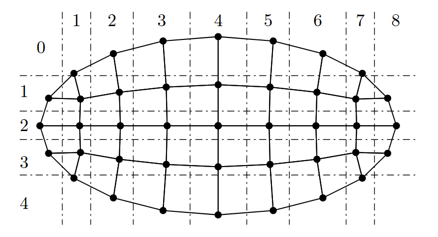
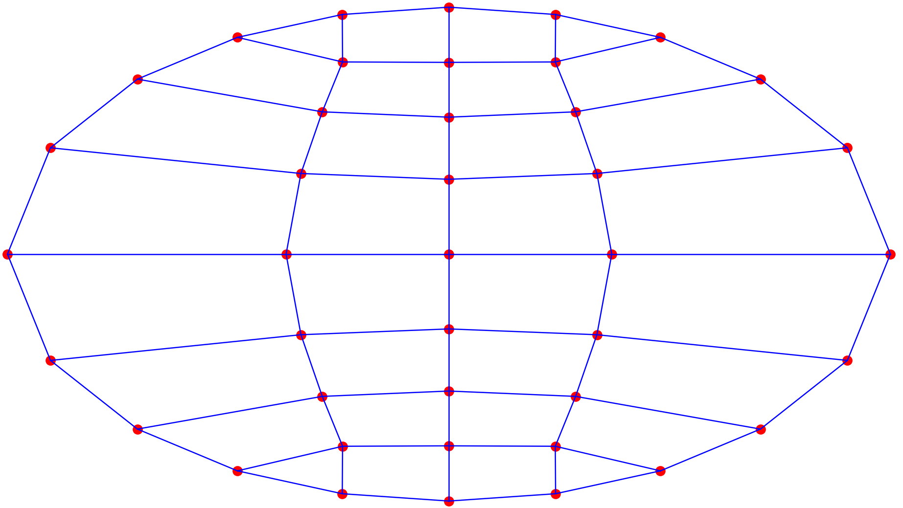
1. 将截面用矩形网格先大致划分为\(c\)列\(r\)行的网格单元，图中为8列4行
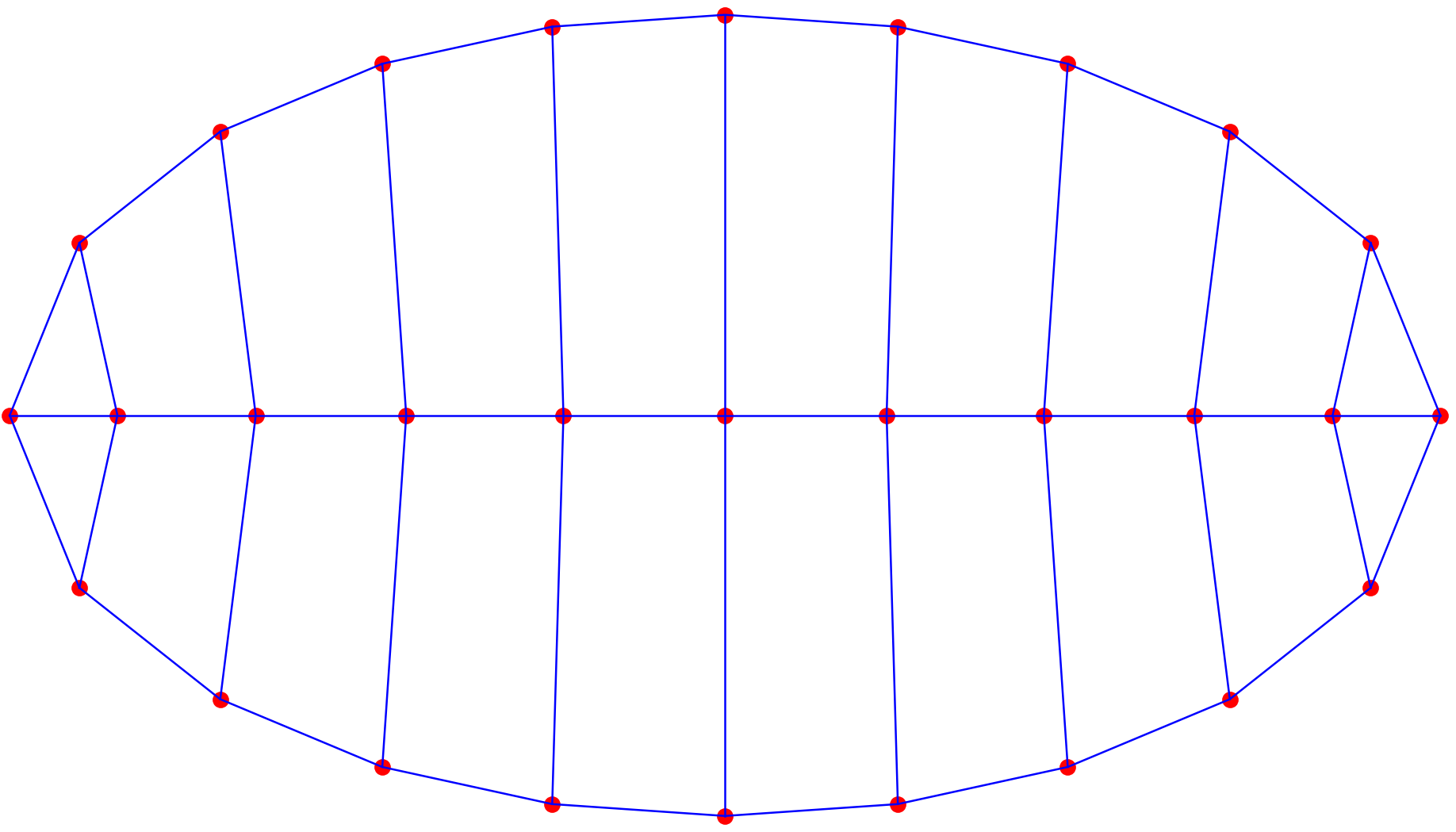
2. 截面的外轮廓线进行等间距划分
3. 对截面内部的节点进行双线性插值计算
4. 按照逆时针的单元局部节点连接顺序，截面角点处拼接为三角形单元，其余部分拼接为四边形单元。

Figure 1: 来自Sherburn博士论文 Fig2.10

外轮廓线等距取点

对闭合曲线按照弧长等距取点的方法有很多，可借助Ai辅助编程，这里给出两种情况：

1. 纯Python实现：使用python构建截面，并对截面外轮廓线进行等距取点
2. 基于PythonOcc实现：传入Face（拓扑面），检测Face的外轮廓线，使用内置方法对其等距取点

第一种情况适合刚学习该算法时，做测试使用；第二种方法用于基于PythonOcc的项目中对纱线截面进行网格划分。

以椭圆形截面为例，使用纯Python实现的方法，对外轮廓线进行等距取点：

def equal_arclength_points(a, b, n_points, dense=40000):
    """
    Take n_points equally spaced points along the arc length on the ellipse x = a*cos(t), y = b*sin(t)
    """
    # 1) Parameter mesh
    t_grid = np.linspace(0.0, 2.0*np.pi, int(dense) + 1)
    dx = -a * np.sin(t_grid)
    dy =  b * np.cos(t_grid)
    v = np.sqrt(dx*dx + dy*dy)

    # 2) Cumulative arc length (composite trapezoidal)
    dt = t_grid[1] - t_grid[0]
    s = np.zeros_like(t_grid)
    k = 1
    while k < t_grid.size:
        s[k] = s[k-1] + 0.5 * (v[k-1] + v[k]) * dt
        k = k + 1
    total_len = s[-1]

    # 3) Equal arc length target
    targets = (np.arange(n_points) * total_len) / float(n_points)

    # 4) Linearly backtrack t(target) and provide coordinates
    t_vals = np.zeros(n_points)
    i = 0
    while i < n_points:
        si = targets[i]
        j = int(np.searchsorted(s, si))
        if j <= 0:
            t_vals[i] = t_grid[0]
        elif j >= s.size:
            t_vals[i] = t_grid[-1]
        else:
            s0 = s[j-1]; s1 = s[j]
            t0 = t_grid[j-1]; t1 = t_grid[j]
            w = (si - s0) / (s1 - s0)
            t_vals[i] = t0 + w * (t1 - t0)
        i = i + 1

    x = a * np.cos(t_vals)
    y = b * np.sin(t_vals)
    pts = np.stack([x, y], axis=1)
    return pts

使用PythonOcc的内置方法对截面外轮廓线进行等距取点：

def equal_arclength_points(face, n_points, O, E1, E2):
    """
    face: Topological Surface
    O: Origin of the local coordinate system of the cross-section
    E1: X-axis of the local coordinate system of the cross-section
    E2: Y-axis of the local coordinate system of the cross-section
    """
    outer = breptools.OuterWire(face)
    comp  = BRepAdaptor_CompCurve(outer)
    # 返回首尾参数(0,1)
    u0, u1 = comp.FirstParameter(), comp.LastParameter()

    O  = np.asarray(O,  dtype=float)
    E1 = np.asarray(E1, dtype=float); E1 /= max(np.linalg.norm(E1), 1e-15)
    E2 = np.asarray(E2, dtype=float); E2 /= max(np.linalg.norm(E2), 1e-15)

    def proj(P3):
        p = np.array([P3.X(), P3.Y(), P3.Z()], dtype=float)
        r = p - O
        return float(np.dot(r, E1)), float(np.dot(r, E2))

    # 计算弧长
    L = GCPnts_AbscissaPoint.Length(comp, u0, u1)
    step = L / float(n_points)

    pts = np.zeros((n_points, 2), dtype=float)
    for i in range(n_points):
        s = step * i
        # 以u0为起点的曲线等分点
        upar = GCPnts_AbscissaPoint(comp, s, u0).Parameter()
        u, v = proj(comp.Value(upar))
        pts[i, 0], pts[i, 1] = u, v

    return pts

上述程序是以外轮廓线（参数化后）的起点进行等距取样，若要以E1为起点，可以稍作修改程序，这里的E1指的是截面所在的局部坐标系的坐标轴，这在后续的细观建模推文中会做出详细解释。

def equal_arclength_points(face, n_points, O, E1, E2):
    outer = breptools.OuterWire(face)
    comp  = BRepAdaptor_CompCurve(outer)
    u0, u1 = comp.FirstParameter(), comp.LastParameter()

    O  = np.asarray(O,  dtype=float)
    E1 = np.asarray(E1, dtype=float); E1 /= max(np.linalg.norm(E1), 1e-15)
    E2 = np.asarray(E2, dtype=float); E2 /= max(np.linalg.norm(E2), 1e-15)

    def proj(P3):
        p = np.array([P3.X(), P3.Y(), P3.Z()], dtype=float)
        r = p - O
        return float(np.dot(r, E1)), float(np.dot(r, E2))

    L = GCPnts_AbscissaPoint.Length(comp, u0, u1)
    step = L / float(n_points)

    # 第一步：先采集所有点
    all_pts = []
    for i in range(n_points):
        s = step * i
        upar = GCPnts_AbscissaPoint(comp, s, u0).Parameter()
        u, v = proj(comp.Value(upar))
        all_pts.append((u, v))

    # 第二步：找到最接近E1方向的点作为起点
    all_pts = np.array(all_pts)
    angles = np.arctan2(all_pts[:, 1], all_pts[:, 0])  # 计算各点角度
    start_idx = np.argmin(np.abs(angles))  # 找到角度最接近0的点

    # 第三步：重新排列点，以E1方向为起点
    pts = np.zeros((n_points, 2), dtype=float)
    for i in range(n_points):
        idx = (start_idx + i) % n_points
        pts[i] = all_pts[idx]

    return pts

上面代码中是以截面局部坐标系的E1轴与截面的交点为起点进行等距取样，这样做的目的是为了后续进行网格拉伸节点拓扑一致，这个细节在后面继续推送【三维结构化网格】再细说。

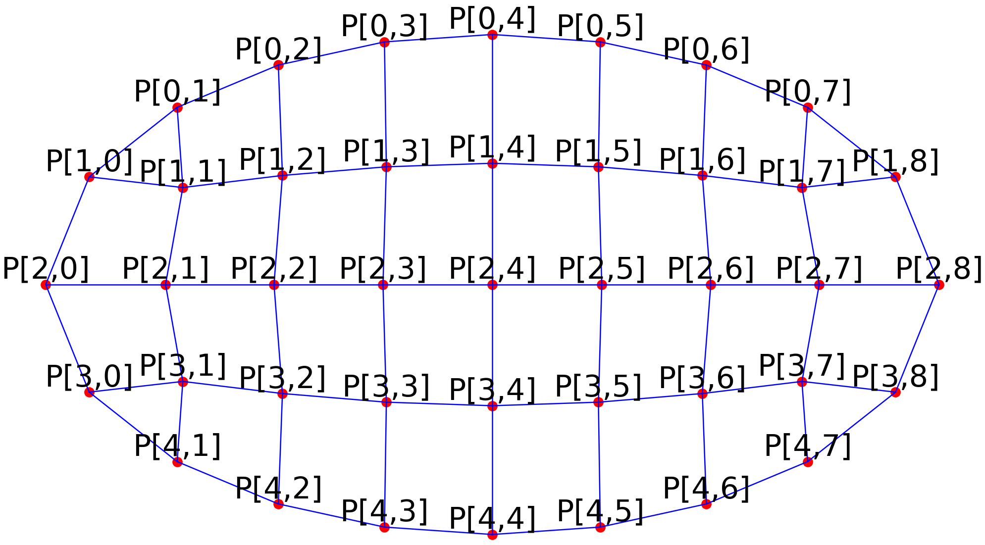
截面外轮廓点进行等距取样后，可对这些点按照一种规则进行标记，方便后续的计算，比如：P[i, j, 0]表示第\(i\)行第\(j\)列节点的\(x\)坐标；P[i, j, 1]表示第\(i\)行第\(j\)列节点的\(y\)坐标。

def map_boundary_points(pts, r, c):
    n = 2 * (r + c) - 4 # n表示等距点的数量
    P = np.full((r + 1, c + 1, 2), np.nan, dtype=float)

    idxs = []
    imid = r // 2

    # 第1步：从右边界中点开始
    idxs.append((imid, c))

    # 第2步：向上遍历右边界（从imid-1到1）
    i = imid - 1
    while i >= 1:
        idxs.append((i, c))
        i = i - 1

    # 第3步：向左遍历上边界（从c-1到1）
    j = c - 1
    while j >= 1:
        idxs.append((0, j))
        j = j - 1

    # 第4步：向下遍历左边界（从1到r-1）
    i = 1
    while i <= r - 1:
        idxs.append((i, 0))
        i = i + 1

    # 第5步：向右遍历下边界（从1到c-1）
    j = 1
    while j <= c - 1:
        idxs.append((r, j))
        j = j + 1

    # 第6步：向上遍历右边界剩余部分（从r-1到imid+1）
    i = r - 1
    while i >= imid + 1:
        idxs.append((i, c))
        i = i - 1

    idxs = np.asarray(idxs, dtype=int)

    k = 0
    while k < n:
        i = int(idxs[k, 0])
        j = int(idxs[k, 1])
        P[i, j, 0] = float(pts[k, 0])
        P[i, j, 1] = float(pts[k, 1])
        k = k + 1

    return P

内部节点双线性插值计算

所谓的“双线性插值计算”，就是考虑横向、纵向的因素对内部节点进行定位，具体可分为两步：

1. 定义两个 辅助点集：\(A_{ij}\)和\(B_{ij}\)，用于确定内部节点位于哪个矩形背景网格中
2. 计算 权重系数，用于确定节点在网格中如何偏移。

\(A_{ij}\)点集-水平方向插值：

• 在第\(i\)行上，从左边界\(P_{i0}\)到右边界\(P_{ic}\)线性插值：

$$ \mathbf { A } _ { i j } \; \; = \; \; \mathbf { P } _ { i 0 } + \frac { j } { c } ( \mathbf { P } _ { i c } - \mathbf { P } _ { i 0 } ) $$ \(B_{ij}\)点集-竖直方向插值：

• 在第\(j\)列上，从上边界\(P_{0j}\)到右边界\(P_{rj}\)线性插值：

\[ \mathbf { B } _ { i j } \; \; = \; \; \mathbf { P } _ { 0 j } + \frac { i } { r } \big ( \mathbf { P } _ { r j } - \mathbf { P } _ { 0 j } \big ) \]

计算权重系数：

\[ d _ { A i j } = \left\| P _ { i 0 } - P _ { i c } \right\| \left( { \frac { 1 } { 2 } } - \left| { \frac { i } { r } } - { \frac { 1 } { 2 } } \right| \right) \]

\[ d _ { B i j } = \left\| P _ { 0 j } - P _ { r j } \right\| \left( { \frac { 1 } { 2 } } - \left| { \frac { j } { c } } - { \frac { 1 } { 2 } } \right| \right) \]

\[ w _ { A i j } = \frac { d _ { B i j } } { d _ { A i j } + d _ { B i j } },\quad w _ { B i j } = \frac { d _ { A i j } } { d _ { A i j } + d _ { B i j } } \]

最终节点位置：

\[ \begin{array} { c c l } { \mathbf { P } _ { i j } } & { = } & { w _ { A i j } \mathbf { A } _ { i j } + w _ { B i j } \mathbf { B } _ { i j } } \end{array} \]

def internal_nodes(P):
    r = P.shape[0] - 1
    c = P.shape[1] - 1

    i = 1 # 从第一行开始
    while i <= r - 1: 
        j = 1 # 从第一列开始
        while j <= c - 1:
            Pi0x, Pi0y = P[i, 0, 0], P[i, 0, 1] # 第i行左边界点
            Picx, Picy = P[i, c, 0], P[i, c, 1] # 第i行右边界点  
            P0jx, P0jy = P[0, j, 0], P[0, j, 1] # 第j列上边界点
            Prjx, Prjy = P[r, j, 0], P[r, j, 1] # 第j列下边界点

            # 在i行上，从左边界到右边界的线性插值点
            tj = j / float(c)
            Aijx = Pi0x + tj * (Picx - Pi0x) # x方向线性插值
            Aijy = Pi0y + tj * (Picy - Pi0y) # y方向线性插值

            # 在j列上，从上边界到下边界的线性插值点。
            ti = i / float(r)
            Bijx = P0jx + ti * (Prjx - P0jx) # x方向线性插值
            Bijy = P0jy + ti * (Prjy - P0jy) # y方向线性插值

            LA = np.sqrt((Picx - Pi0x)**2 + (Picy - Pi0y)**2) # 第i行左右边界长度
            LB = np.sqrt((Prjx - P0jx)**2 + (Prjy - P0jy)**2) # 第j列上下边界长度
            dA = (0.5 - abs(tj - 0.5)) * LA # 水平方向有效距离
            dB = (0.5 - abs(ti - 0.5)) * LB # 垂直方向有效距离

            denom = dA + dB
            if denom == 0.0:
                wA = 0.5
                wB = 0.5
            else:
                wA = dB / denom
                wB = dA / denom

            P[i, j, 0] = wA * Aijx + wB * Bijx
            P[i, j, 1] = wA * Aijy + wB * Bijy

            j = j + 1
        i = i + 1

    return P

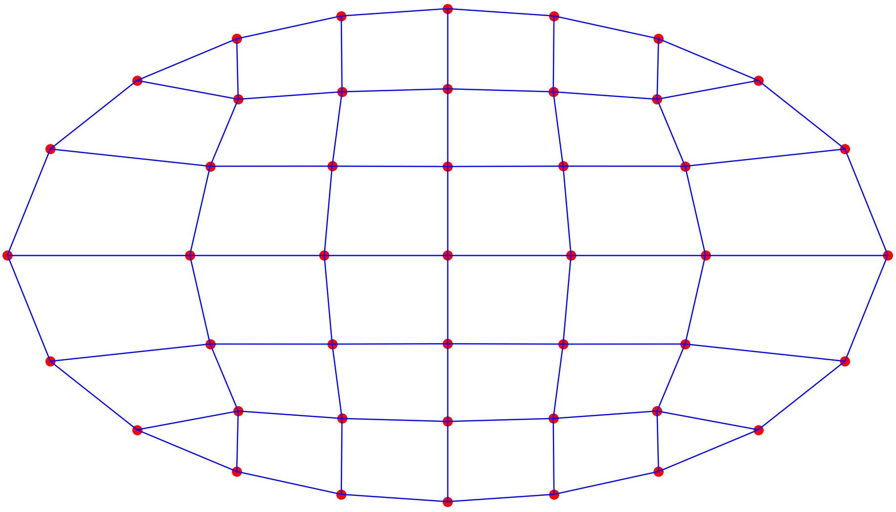
数值算例

以椭圆截面为例，调节不同的\(r\)、\(c\)值，控制单元密度。

• 
• 
• 
• 
• 
• 

---

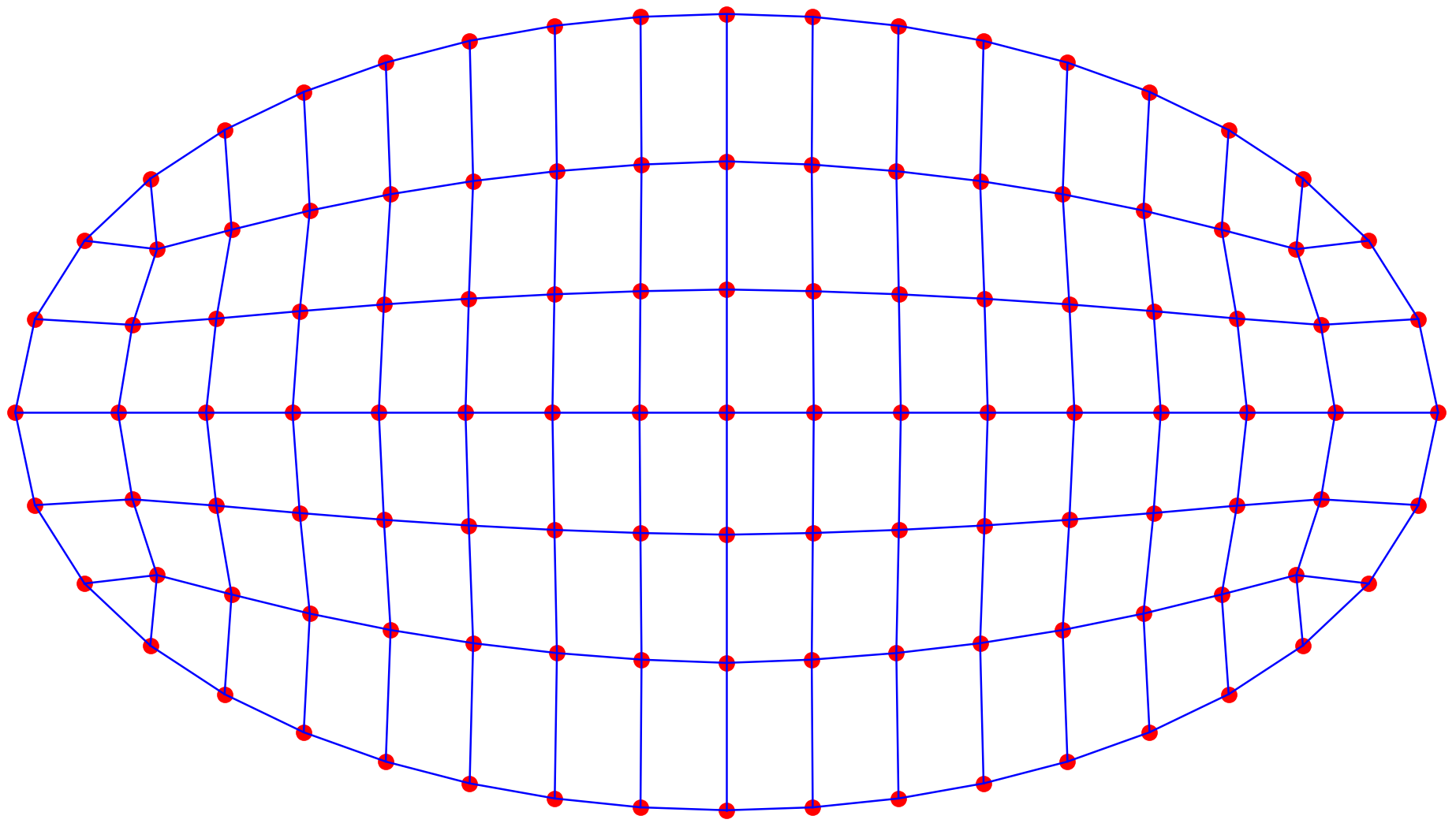
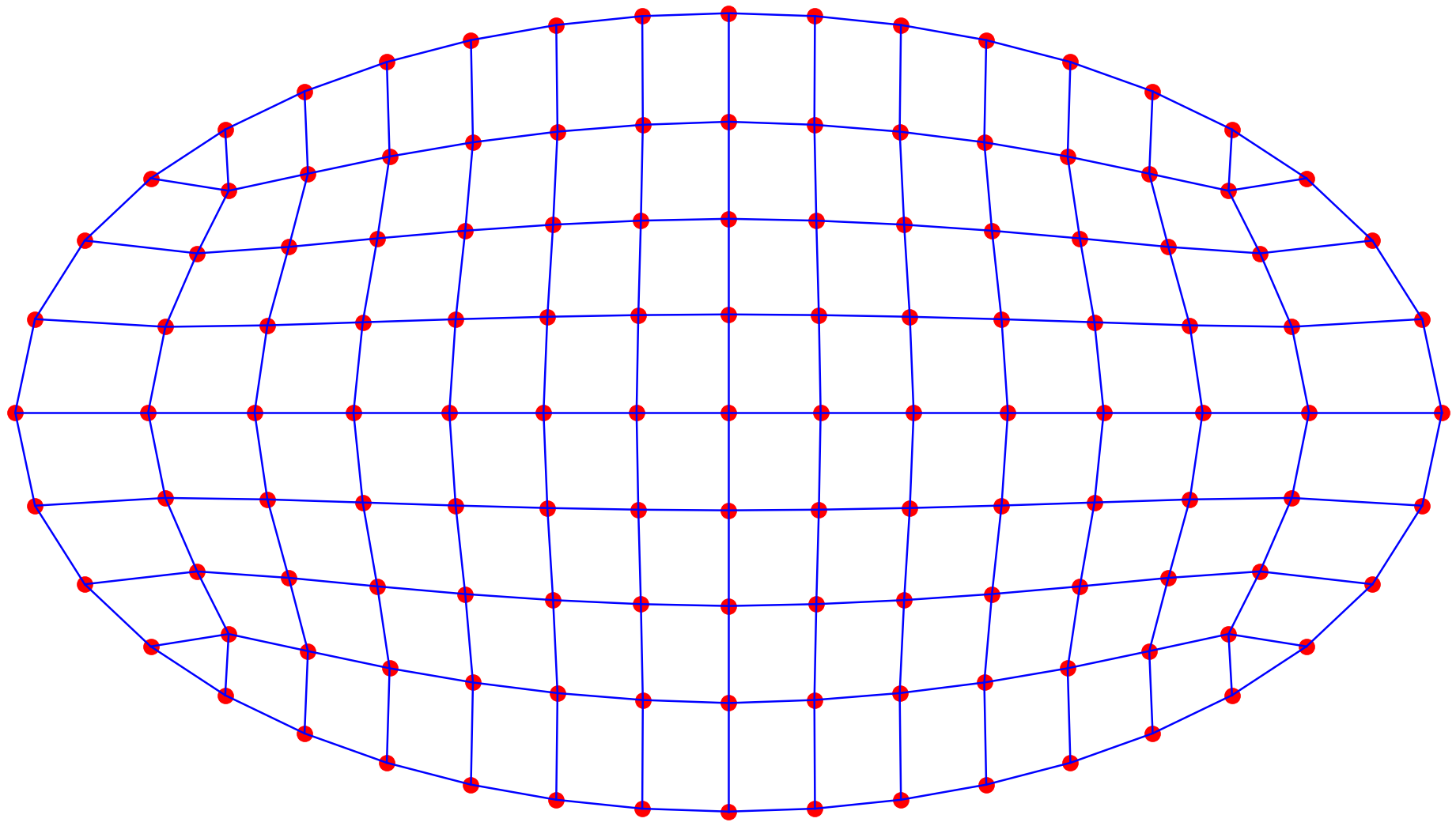
注：

1. 本次分享的网格算法为木木按照论文上的解释加以自己理解进行分享，若有不当之处，欢迎私信、留言讨论；
2. 算例中使用的是椭圆型截面，对于圆形、幂椭圆、透镜型等截面类型也都适用，感兴趣的小伙伴可在此程序的基础上更换其他截面进行尝试。