Vedo库
约 397 个字 111 行代码 4 张图片 预计阅读时间 3 分钟
Vedo是一个用于3D可视化和网格处理的Python库,与Pyvista类似。它们都基于VTK(Visualization Toolkit),提供强大的后处理渲染功能。本节将介绍如何在有限元后处理工作中利用Vedo库。
首先,先pip安装vedo:pip install vedo。
具体参数说明及案例可在官网:https://vedo.embl.es。
创建Mesh对象
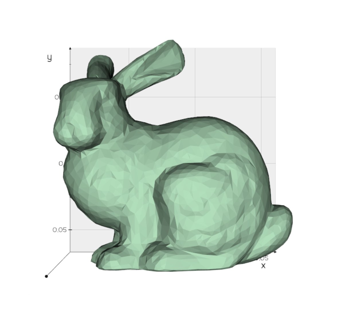
以有限元网格信息为例,假设已经从Abaqus的inp文件中已经解析出节点单元信息,现在如何使用vedo库进行可视化:
from vedo import *

nodes = [
    [0, 0, 0],
    [1, 0, 0],
    [1, 1, 0],
    [0, 1, 0],
]
elements = [
    [0, 1, 2],
    [0, 2, 3],
]
# 创建mesh
mesh = Mesh([nodes, elements]).lc('orange').lw(1)

plt = Plotter()
plt.show(mesh, axes=1)
通过上面格式的转化,就可以创建vedo库的Mesh对象了,后续的所有操作都基于该对象。
用户也可通过导入vtk格式文件来创建对象:mesh = load("CRACK.vtk")。
云图绘制基础
场变量信息
使用已有的节点单元数据创建Mesh对象后,可以直接绘制出网格模型,场变量信息需要添加进Mesh对象中。
# 位移场 (每个节点的 [dx, dy, dz])
displacements = [
    [0.1, 0.2, 0.2],
    [0.0, 0.3, 0.0],
    [-0.1, 0.2, 0.0],
    [0.0, -0.1, 0.1],
]

Umag = mag(displacements)

# 添加标量数据到网格点
mesh.pointdata["Displacement Magnitude"] = displacements
导入vtk的方法创建Mesh对象时可以直接索引vtk文件中的节点场数据信息。
# vtk文件中位移场对应的label为Displacement
displacement = mesh.pointdata["Displacement"]
# U1
U1 = displacement[:,0]
查询Mesh信息
常用的查询方法总结如下:
# Print the points and faces of the mesh as numpy arrays
print('vertices:', mesh.vertices) # same as mesh.points or mesh.coordinates
print('faces   :', mesh.cells)

print("Number of nodes:", mesh.npoints) # 或者.nvertices
print("Number of elements:", mesh.ncells)
print("Cell connectivity of elements:", mesh.cells)
print("Center of elements:", mesh.cell_centers)

print("Available point data:", mesh.pointdata.keys())  # 输出节点场数据label
print("Available cell data:", mesh.celldata.keys())    # 输出单元场数据label
模型风格
mesh.lw(1) # 线宽
mesh.c('purple5') # 单元面颜色
mesh.lc('b') # 线颜色
mesh.alpha(0.5) # 透明度

mesh.wireframe().c("yellow")# wireframe,并设置其线条颜色
plt.render_hidden_lines # 隐藏单元边界
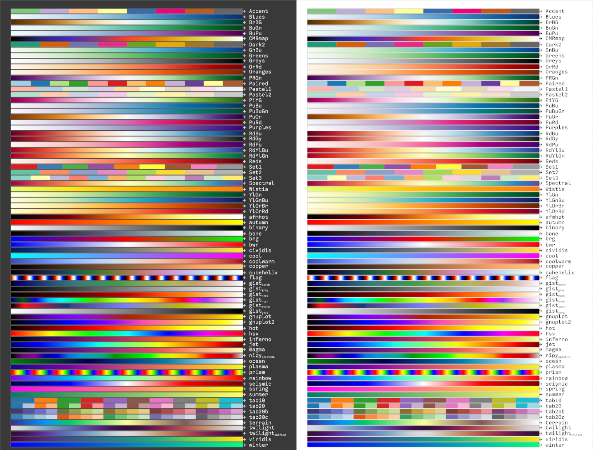
cmap
vedo库支持的cmap种类:
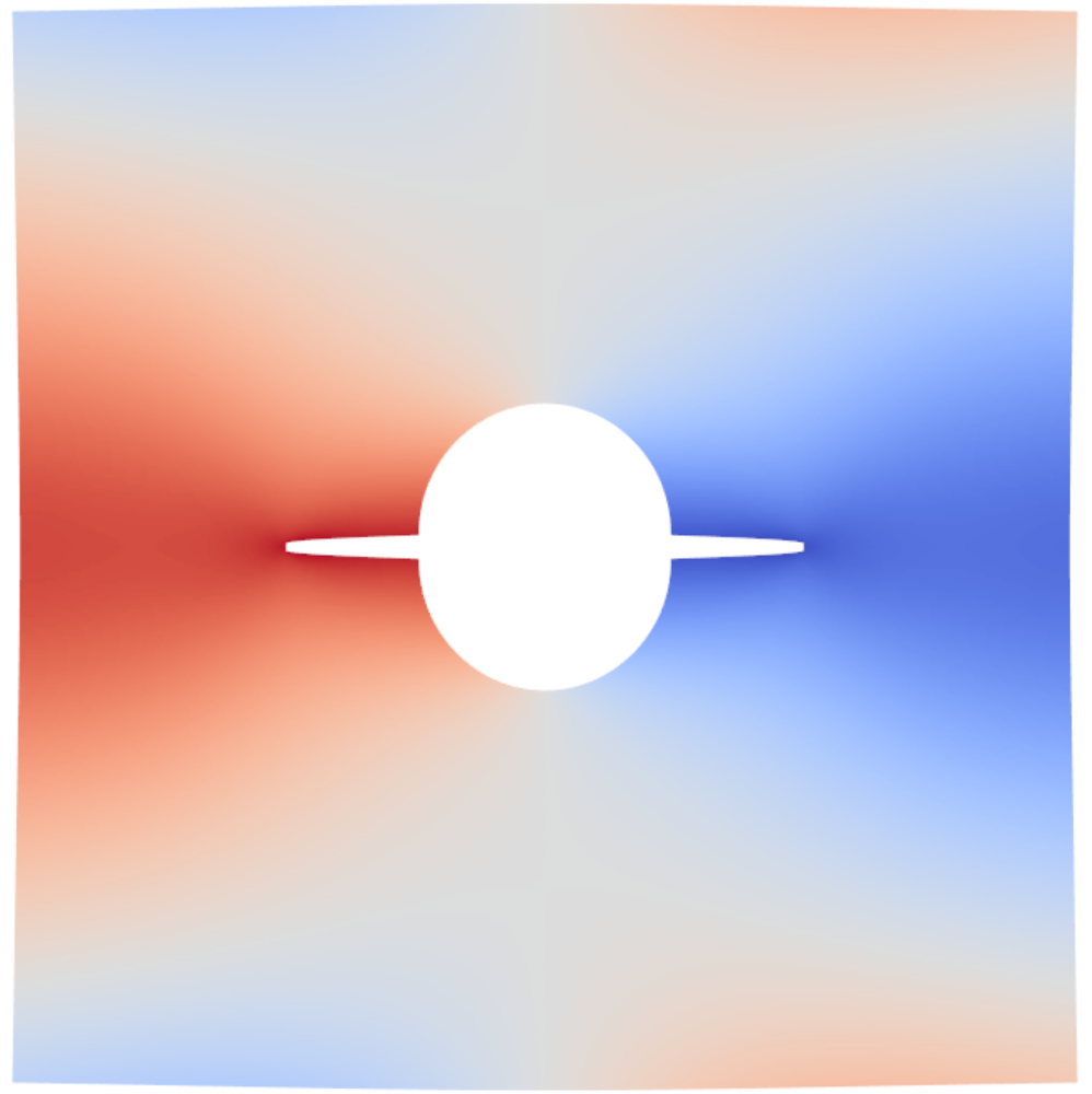
说了这么久,先整个云图吧,直接案例教学。
from vedo import *

mesh = load("CRACK.vtk")
displacement = mesh.pointdata["U"]
U1 = displacement[:, 0]

mesh.cmap("coolwarm", U1, on="points")
show(mesh)
现在来看一下cmap函数的用法,基本用法注释中已标明。
def cmap(
    self,
    input_cmap, # cmap name
    input_array=None, # 场变量
    on='', # (str) either 'points' or 'cells' or blank (automatic). Apply the color map to data which is defined on either points or cells
    n_colors=256, # (int) number of distinct colors to be used in colormap table.
    alpha=1.0, # 透明度
)
自定义colorbar
(个人感觉:Pyvista更好用一些)
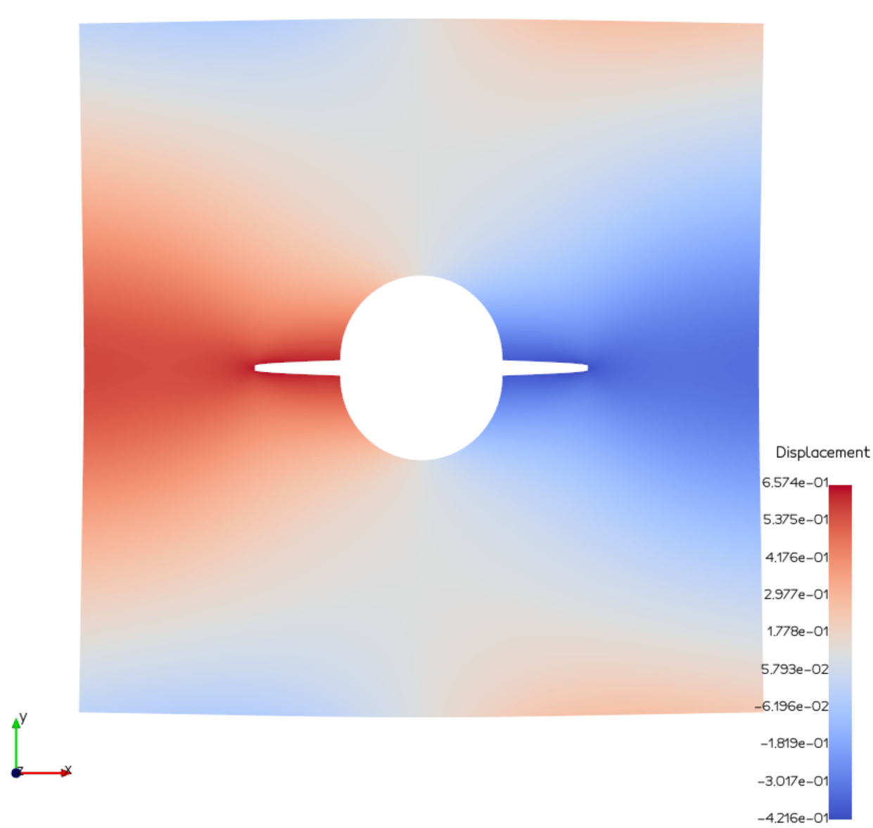
def ScalarBar(
    obj,
    title="", # (str) scalar bar title
    pos=(), # (list) position coordinates of the bottom left corner. Can also be a pair of (x,y) values in the range [0,1] to indicate the position of the bottom-left and top-right corners.
    size=(80, 400), # (float,float) size of the scalarbar in number of pixels (width, height)
    font_size=14, # (float) size of font for title and numeric labels
    title_yoffset=20, # (float) vertical space offset between title and color scalarbar
    nlabels=None, # (int) number of numeric labels
    c="k", # (list) color of the scalar bar text
    horizontal=False, #  (bool) lay the scalarbar horizontally
    use_alpha=True, # (bool) render transparency in the color bar itself
    label_format=":6.3g", # (str) c-style format string for numeric labels
)
绘图进阶
节点单元label
point_ids = mesh.labels('id', on="points").c('green')
cell_ids  = mesh.labels('id', on="cells" ).c('black')
show(mesh, point_ids, cell_ids)
缩放因子
缩放的同时,节点坐标也在跟着缩放。
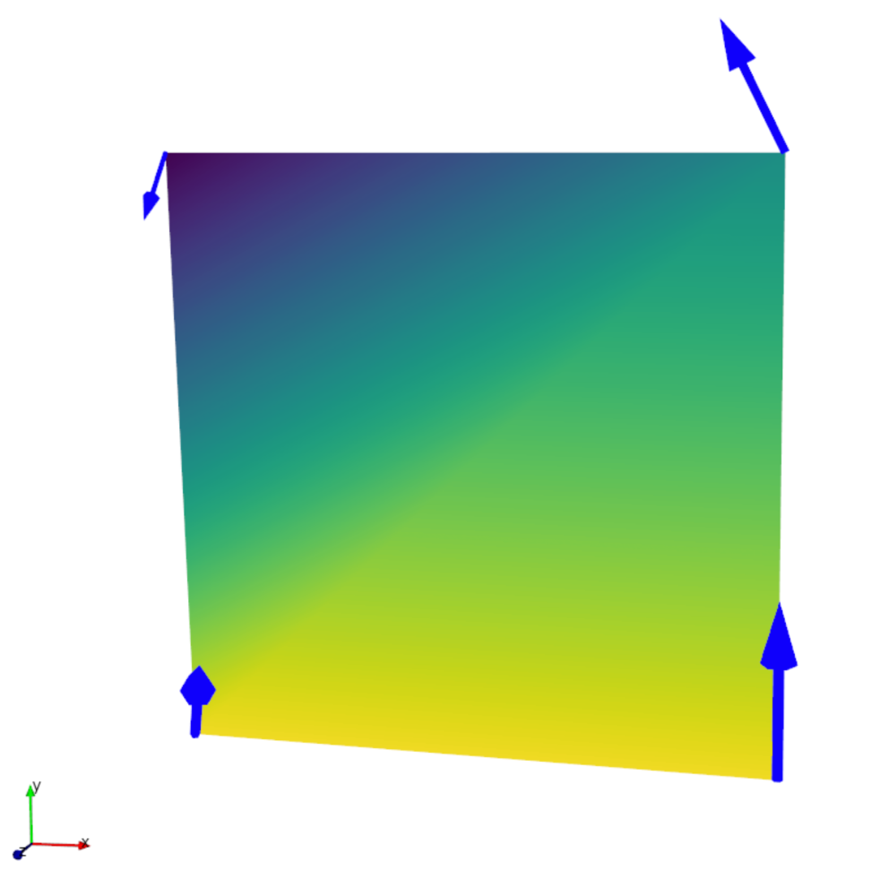
矢量箭头绘制
# 创建位移矢量箭头
arrows = Arrows(
    np.array(nodes),                # 起点
    np.array(nodes) + np.array(displacements),  # 终点
    c="blue",
)

# 显示结果
show(mesh, arrows, axes=4)
Arrows(
    start_pts, # 箭头的起点坐标列表,例如 `[[x1, y1, z1], [x2, y2, z2]]`。
    end_pts, # 箭头的终点坐标列表。如果为 `None`,则箭头方向由 `start_pts` 和缩放因子 `s` 决定。
    s=None, # 当 `end_pts=None` 时,指定箭头方向矢量的缩放因子。默认值为 1。
    shaft_radius=None, # 箭头轴的半径。默认值为自动计算的值,约为箭头长度的 5%。
    head_radius=None, # 箭头头部的半径。默认值为自动计算的值,约为轴半径的两倍。
    head_length=None, # 箭头头部的长度。默认值为自动计算的值,约为箭头长度的 15%。
    thickness=1.0, # 箭头的厚度比率(非圆柱形箭头)。
    res=6, # 箭头的分辨率,控制轴和头部的多边形细节,默认值为 6。
    c='k3', # 箭头的颜色,支持单一颜色或每个箭头不同颜色(与cmap颜色一致:c = "coolwarm")。
    alpha=1.0 # 箭头的透明度,取值范围为 `[0, 1]`。
)